!gdalinfo --versionGDAL 3.7.3, released 2023/10/30When making Cloud-Optimized GeoTIFFs (COGs), you can select the resampling method to generate the overviews. Different types of data (e.g., nominal, ordinal, discrete, continuous) can drastically change appearance when more zoomed out based on the chosen method. This is most important when using software that renders from overviews (e.g., QGIS, ArcGIS), particularly web tilers like Titiler.
Also, when using a tiling service on a high-resolution dataset, you will often have many tiles of source data. The idea behind this notebook is that before you generate all your final output data, as COGs, or if you need to rebuild your overviews, you should first test on some representative samples. After testing, you’ll know which method to use in your data pipeline.
This notebook loops over the overview resampling methods available in GDAL applying it to the same sample tile to compare how the dataset will appear when zoomed out from the full resolution.
Note: GDAL 3.2 specifically added the ability to specify the resampling method for the overviews. GDAL 3.3 added a couple of new resampling ways.
gdal >= 3.2 for Overview Resampling to workThe packages needed for this notebook can be installed with conda or mamba. Using the environment.yml from this folder run:
conda env create -f environment.ymlOr:
mamba env create -f environment.ymlOr you can install the packages you need manually:
mamba create -q -y -n coguide-cog -c conda-forge 'gdal>=3.3' 'rasterio>=1.3.3' 'rio-cogeo=3.5.0' ipykernel matplotlib earthaccessThen, you may activate and select the kernel in the notebook (running in Jupyter):
conda activate coguide-cogThis notebook has been tested to work with the listed Conda environment.
Remember to switch your notebook kernel if you made a new env; you may need to activate the new env first.
First, we should verify our GDAL version:
!gdalinfo --versionGDAL 3.7.3, released 2023/10/30import os
import earthaccess
import matplotlib.pyplot as plt
import rasterio as rio
from rasterio.session import AWSSession
from rasterio.plot import show
from rio_cogeo import cog_translate, cog_profiles/home/ochotona/anaconda3/envs/coguide-cog/lib/python3.11/site-packages/tqdm/auto.py:21: TqdmWarning: IProgress not found. Please update jupyter and ipywidgets. See https://ipywidgets.readthedocs.io/en/stable/user_install.html
from .autonotebook import tqdm as notebook_tqdmThe example data comes from the Aboveground Biomass Density for High Latitude Forests from ICESat-2, 2020
To access and integrate NASA Earth data into your Jupyter Notebook, you can create an account by visiting NASA’s Earthdata Login page. This will enable you to register for an account and retrieve the datasets used in the notebook.
You can see the whole mosaic of all the data on the MAAP Biomass dashboard
For this example, we will pull a single 3000x3000 pixel tile that is part of the larger dataset of more than 3500 tiles.
We must retrieve a NASA Earth data session for downloading data:
earthaccess.login(strategy="interactive")<earthaccess.auth.Auth at 0x7faa304b5e10>We can now query NASA CMR to retrieve a download URL:
short_name = 'Boreal_AGB_Density_ICESat2_2186'
item = 'Boreal_AGB_Density_ICESat2.boreal_agb_202302061675666220_3741.tif'

item_results = earthaccess.search_data(
    short_name=short_name,
    cloud_hosted=True,
    granule_name=item

)
Granules found: 1Finally, we can download the COG for local use:
test_data_dir = "./test_data"
os.makedirs(test_data_dir, exist_ok=True)

sample_files = earthaccess.download(item_results, test_data_dir)
tile = f"{sample_files[0]}"
Getting 1 granules, approx download size: 0.09 GBQUEUEING TASKS | : 100%|██████████| 2/2 [00:00<00:00, 1733.18it/s]File boreal_agb_202302061675666220_3741.tif already downloaded
File boreal_agb_202302061675666220_3741.tif.sha256 already downloadedPROCESSING TASKS | : 100%|██████████| 2/2 [00:00<00:00, 15621.24it/s]
COLLECTING RESULTS | : 100%|██████████| 2/2 [00:00<00:00, 34239.22it/s]Note: We downloaded the file because, it’s small (less than 100 MB), and we’re going to use the whole file several times.
Using rio cogeo, we can investigate if the file has tiles and what resampling was used:
!rio cogeo info {tile}Driver: GTiff File: /home/ochotona/code/devseed/cloud-optimized-geospatial-formats-guide/cloud-optimized-geotiffs/test_data/boreal_agb_202302061675666220_3741.tif COG: True Compression: LZW ColorSpace: None Profile Width: 3000 Height: 3000 Bands: 2 Tiled: True Dtype: float32 NoData: -9999.0 Alpha Band: False Internal Mask: False Interleave: PIXEL ColorMap: False ColorInterp: ('gray', 'undefined') Scales: (1.0, 1.0) Offsets: (0.0, 0.0) Geo Crs: PROJCS["unnamed",GEOGCS["GRS 1980(IUGG, 1980)",DATUM["unknown",SPHEROID["GRS80",6378137,298.257222101],TOWGS84[0,0,0,0,0,0,0]],PRIMEM["Greenwich",0],UNIT["degree",0.0174532925199433,AUTHORITY["EPSG","9122"]]],PROJECTION["Albers_Conic_Equal_Area"],PARAMETER["latitude_of_center",40],PARAMETER["longitude_of_center",180],PARAMETER["standard_parallel_1",50],PARAMETER["standard_parallel_2",70],PARAMETER["false_easting",0],PARAMETER["false_northing",0],UNIT["metre",1,AUTHORITY["EPSG","9001"]],AXIS["Easting",EAST],AXIS["Northing",NORTH]] Origin: (1448521.9999999953, 2853304.0000000093) Resolution: (30.0, -30.0) BoundingBox: (1448521.9999999953, 2763304.0000000093, 1538521.9999999953, 2853304.0000000093) MinZoom: 7 MaxZoom: 11 Image Metadata AREA_OR_POINT: Area Image Structure COMPRESSION: LZW INTERLEAVE: PIXEL Band 1 Description: aboveground_biomass_density (Mg ha-1) ColorInterp: gray Metadata: STATISTICS_MAXIMUM: 347.71490478516 STATISTICS_MEAN: 44.388942987808 STATISTICS_MINIMUM: 2.5594062805176 STATISTICS_STDDEV: 30.371053229248 STATISTICS_VALID_PERCENT: 86.55 Band 2 Description: standard_deviation ColorInterp: undefined Metadata: STATISTICS_MAXIMUM: 121.33344268799 STATISTICS_MEAN: 6.1550359252236 STATISTICS_MINIMUM: 0.25763747096062 STATISTICS_STDDEV: 3.7940122373131 STATISTICS_VALID_PERCENT: 86.55 IFD Id Size BlockSize Decimation 0 3000x3000 256x256 0 1 1500x1500 128x128 2 2 750x750 128x128 4 3 375x375 128x128 8
Now, let’s generate overviews with each resampling method possible in GDAL.
def generate_overview(src_path: str, out_dir: str, resample_method: str) -> str:
    '''
    Create a copy of original GeoTiff as COG with different overview resampling method
    src_path = the original GeotTiff
    out_dir = the folder for outputs (can differ from src)
    method = the resampling method
    return = the path to the new file
    '''
    #make sure the output folder exists
    os.makedirs(out_dir, exist_ok=True)
    dst_path = src_path.replace(".tif", f"_{resample_method}.tif")
    dst_path = f"{out_dir}/{os.path.basename(dst_path)}"

    # Using multiple CPUS
    # Using blocksize 512 per recommendations
    config = {"GDAL_NUM_THREADS": "ALL_CPUS", "GDAL_TIFF_OVR_BLOCKSIZE": "512"}
    output_profile = cog_profiles.get("deflate")
    output_profile.update({"blockxsize": "512", "blockysize": "512"})

    print(f"Creating COG using '{resample_method}' method: {dst_path}")
    cog_translate(
        src_path,
        dst_path,
        output_profile,
        config=config,
        overview_resampling=resample_method,
        forward_band_tags=True,
        use_cog_driver=True,
        quiet=True,
    )

    return dst_path
Now, we can make a list of the resampling methods offered by GDAL. Some resampling methods aren’t appropriate for the data, so we are doing to drop those from the list. You can see descriptions at https://gdal.org/programs/gdalwarp.html#cmdoption-gdalwarp-r
# Make a list of resampling methods that GDAL 3.4+ allows

from rasterio.enums import Resampling

# Drop some irrelevant methods
excluded_resamplings = {
    Resampling.max,
    Resampling.min,
    Resampling.med,
    Resampling.q1,
    Resampling.q3,
}
overview_resampling_methods = [method for method in Resampling if method not in excluded_resamplings]
resample_methods = [method.name for method in overview_resampling_methods]
print(resample_methods)
['nearest', 'bilinear', 'cubic', 'cubic_spline', 'lanczos', 'average', 'mode', 'gauss', 'sum', 'rms']For each resampling method, we can create a copy of the data with it’s given overview method:
files = [generate_overview(tile, test_data_dir, resample_method) for resample_method in resample_methods] Creating COG using 'nearest' method: ./test_data/boreal_agb_202302061675666220_3741_nearest.tif
Creating COG using 'bilinear' method: ./test_data/boreal_agb_202302061675666220_3741_bilinear.tif
Creating COG using 'cubic' method: ./test_data/boreal_agb_202302061675666220_3741_cubic.tif
Creating COG using 'cubic_spline' method: ./test_data/boreal_agb_202302061675666220_3741_cubic_spline.tif
Creating COG using 'lanczos' method: ./test_data/boreal_agb_202302061675666220_3741_lanczos.tif
Creating COG using 'average' method: ./test_data/boreal_agb_202302061675666220_3741_average.tif
Creating COG using 'mode' method: ./test_data/boreal_agb_202302061675666220_3741_mode.tif
Creating COG using 'gauss' method: ./test_data/boreal_agb_202302061675666220_3741_gauss.tif
Creating COG using 'rms' method: ./test_data/boreal_agb_202302061675666220_3741_rms.tifWe can validate that the overviews were created:
!rio cogeo info {files[0]}Driver: GTiff File: /home/ochotona/code/devseed/cloud-optimized-geospatial-formats-guide/cloud-optimized-geotiffs/test_data/boreal_agb_202302061675666220_3741_nearest.tif COG: True Compression: DEFLATE ColorSpace: None Profile Width: 3000 Height: 3000 Bands: 2 Tiled: True Dtype: float32 NoData: -9999.0 Alpha Band: False Internal Mask: False Interleave: PIXEL ColorMap: False ColorInterp: ('gray', 'undefined') Scales: (1.0, 1.0) Offsets: (0.0, 0.0) Geo Crs: PROJCS["unnamed",GEOGCS["GRS 1980(IUGG, 1980)",DATUM["unknown",SPHEROID["GRS80",6378137,298.257222101],TOWGS84[0,0,0,0,0,0,0]],PRIMEM["Greenwich",0],UNIT["degree",0.0174532925199433,AUTHORITY["EPSG","9122"]]],PROJECTION["Albers_Conic_Equal_Area"],PARAMETER["latitude_of_center",40],PARAMETER["longitude_of_center",180],PARAMETER["standard_parallel_1",50],PARAMETER["standard_parallel_2",70],PARAMETER["false_easting",0],PARAMETER["false_northing",0],UNIT["metre",1,AUTHORITY["EPSG","9001"]],AXIS["Easting",EAST],AXIS["Northing",NORTH]] Origin: (1448521.9999999953, 2853304.0000000093) Resolution: (30.0, -30.0) BoundingBox: (1448521.9999999953, 2763304.0000000093, 1538521.9999999953, 2853304.0000000093) MinZoom: 7 MaxZoom: 11 Image Metadata AREA_OR_POINT: Area OVR_RESAMPLING_ALG: NEAREST Image Structure COMPRESSION: DEFLATE INTERLEAVE: PIXEL LAYOUT: COG Band 1 Description: aboveground_biomass_density (Mg ha-1) ColorInterp: gray Metadata: STATISTICS_MAXIMUM: 347.71490478516 STATISTICS_MEAN: 44.388942987808 STATISTICS_MINIMUM: 2.5594062805176 STATISTICS_STDDEV: 30.371053229248 STATISTICS_VALID_PERCENT: 86.55 Band 2 Description: standard_deviation ColorInterp: undefined Metadata: STATISTICS_MAXIMUM: 121.33344268799 STATISTICS_MEAN: 6.1550359252236 STATISTICS_MINIMUM: 0.25763747096062 STATISTICS_STDDEV: 3.7940122373131 STATISTICS_VALID_PERCENT: 86.55 IFD Id Size BlockSize Decimation 0 3000x3000 512x512 0 1 1500x1500 512x512 2 2 750x750 512x512 4 3 375x375 512x512 8
Now that we’ve generated each of the overview methods we can plot the full data and each overview. The overviews are labelled by their magnification. Example and overview of 2, is the dimensions divided by 2. Typically in COGs you will keep making overviews until the one of the dimensions is less than 512 pixels.
def compare_overviews(image: str, fig, ax_list, row):
    '''
    Read the original data, and overviews an plot them.
    image = the path to input COG to read
    '''

    with rio.open(image, 'r') as src:
        #Plot the 1st band
        oviews = src.overviews(1)
        #fig, ax_list = plt.subplots(ncols=(len(oviews)+1), nrows=1, figsize=(16,4))
        show(src, ax=ax_list[row, 0])

        bname = os.path.basename(image)
        row_name = bname.split("_")[-1].replace('.tif', '')

        ax_list[row,0].set_title("Full Resolution")
        ax_list[row,0].set_ylabel(row_name)
        ax_list[row,0].xaxis.set_ticklabels([])
        ax_list[row,0].yaxis.set_ticklabels([])

        #increment counter so overviews plot starting in the second column
        k = 1
        for oview in oviews:
            height = int(src.height // oview)
            width = int(src.width // oview)
            thumbnail = src.read(1, out_shape=(1, height, width))
            show(thumbnail, ax=ax_list[row,k])
            ax_list[row,k].set_title(f'{height}x{width}')
            ax_list[row,k].xaxis.set_ticklabels([])
            ax_list[row,k].yaxis.set_ticklabels([])
            k += 1

    return
For each variat, we will add interpretation details below the plot. Notice we are using hard-coded values for the levels:
fig, ax_list = plt.subplots(ncols=4, nrows=len(files), figsize=(16,32), constrained_layout=True)
row = 0
for file in files:
    compare_overviews(file, fig, ax_list, row)
    row += 1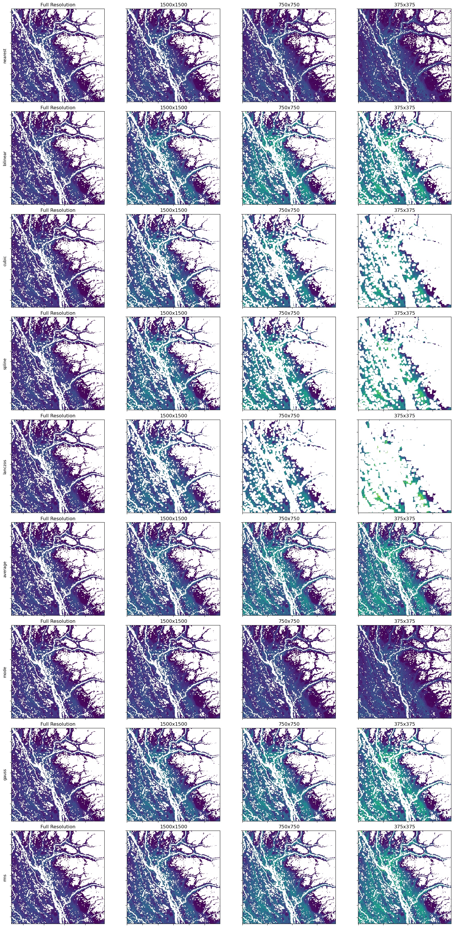
With this particular example, you can see the default method (CUBIC) over-represents the amount of NoData cells as you zoom out (left to right). You can also see how some algorithms hide NoData when zoomed out, and the different methods vary in their level of smoothness.
Depending on what impression you want viewers to get, comparing will help you choose which method to use.